Bump Map Generation
Bump mapping is a texture-based technique that allows improving the lighting model of a 3D renderer. I’m a big fan of bump mapping; I think it’s a great way to really make the graphics of a renderer pop at no additional geometry processing cost.
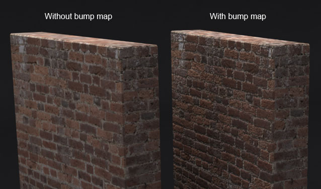
Much has been written about this technique, as it’s widely used in lots of popular games. The basic idea is to perturb normals used for lighting at the per-pixel level, in order to provide additional shading cues to the eye.
The beauty of this technique is that it doesn’t require any additional geometry for the model, just a new texture map containing the perturbed normals.
This post covers the topic of bump map generation, taking as input nothing but a diffuse texture. It is based on the techniques described in the books “More OpenGL” by Dave Astle and “Mathematics for 3D Games And Computer Graphics” by Eric Lengyel.
Let’s get started! Here’s the Imp texture that I normally use in my examples. You might remember the Imp from my Shadow Mapping on iPad post.
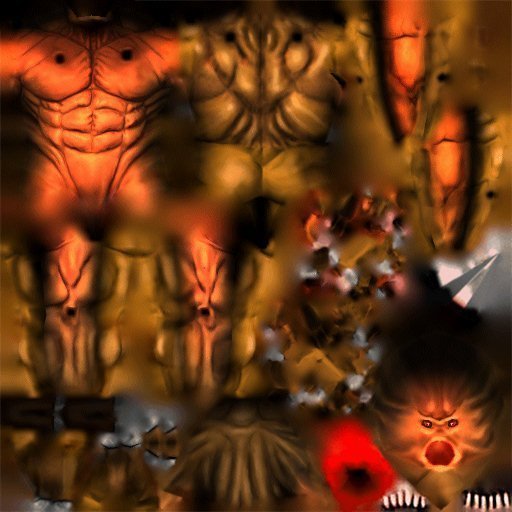
The idea is to generate the bump map from this texture. In order to do this, what we are going to do is analyze the diffuse map as if it were a heightmap that describes a surface. Under this assumption, the bump map will be composed of the surface normals at each point (pixel).
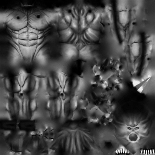
So, the question is, how do we obtain a heightmap from the diffuse texture? We will cheat. We will convert the image to grayscale and hope for the best. At least this way we will be taking into account the contribution of each color channel for each pixel we process.
Let’s call H the heightmap and D the diffuse map. Converting an image to grayscale can be easily done programatically using the following equation:
![\forall (i,j) \in [0..width(D), 0..height(D)], H_{i,j} = red(D_{i,j}) * 0.33 + green(D_{i,j})* 0.66 + blue(D_{i,j}) * 0.11](http://s0.wp.com/latex.php?latex=++%5Cforall+%28i%2Cj%29+%5Cin+%5B0..width%28D%29%2C+0..height%28D%29%5D%2C+H_%7Bi%2Cj%7D+%3D+red%28D_%7Bi%2Cj%7D%29+%2A+0.33+%2B+green%28D_%7Bi%2Cj%7D%29%2A+0.66+%2B+blue%28D_%7Bi%2Cj%7D%29+%2A+0.11++&bg=ffffff&fg=000000&s=0 "\forall (i,j) \in [0..width(D), 0..height(D)], H_{i,j} = red(D_{i,j}) * 0.33 + green(D_{i,j})* 0.66 + blue(D_{i,j}) * 0.11")
As we apply this formula to every pixel, we obtain a grayscale image (our heightmap), shown in the next figure:
Now that we have our heightmap, we will study how the grayscale colors vary in the horizontal 

If 
")
 \\ t_{i,j} = (0, 1, H_{i, j+1}-H_{i,j-1})")

After applying this logic to the entire heightmap, we obtain our bump map.
We must be careful when storing a normalized vector in a texture. Because vector components will be in the [-1,1] range, but values we can store in the bitmap need to be in the [0, 255] range, we will have to convert between both value ranges to store our data as color.
A linear conversion produces an image like the following:
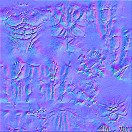
Notice the prominence of blue, which represents normals close to the (unperturbed) ")
We are a bit more interested in the darker areas, however. This is where the normals are more perturbed and will make the Phong equation subtly affect shading, expressing “discontinuities” in the surface that the eye will interpret as “wrinkles”.
Other colors will end up looking like slopes and/or curves.
In all fairness, the image is a bit more grainy than I would’ve liked. We can apply a bilinear filter on it to make it smoother. We could also apply a scale to the
However, since we are going to be interpolating rotated vectors during the rasterization process, these images will be good enough for now.
I’ve written a short Python script that implements this logic and applies it on any diffuse map. It is now part of the Vortex Engine toolset.
In my next post I’m going to discuss how to implement the vertex and fragment shaders necessary to apply bump mapping on a trivial surface. Stay tuned!