Bump Mapping a Simple Surface

In my last post, I started discussing Bump Mapping and showed a mechanism through which we can generate a normal map from any diffuse texture. At the time, I signed off by mentioning next time I would show you how to apply a bump map on a trivial surface. This is what we are going to do today.

 
In the video above you can see the results of the effect we are trying to achieve. This video was generated from a GIF file created using the Vortex Engine. It clearly shows the dramatic lighting effect bump mapping achieves.

Although it may seem as if this image is composed of a detailed mesh of the boss’ head, it is in fact just two triangles. If you could see the image from the side, you’d see it’s completely flat! The illusion of curvature and depth is generated by applying per-pixel lighting on a bump mapped surface.

How does bump mapping work? Our algorithm will take as input two images: the diffuse map and the bump map. The diffuse map is just the colors of each pixel in the image, whereas the bump map consists in an encoded set of per-pixel normals that we will use to affect our lighting equation.

Here’s the diffuse map of the Boss door:

And here’s the bump map:

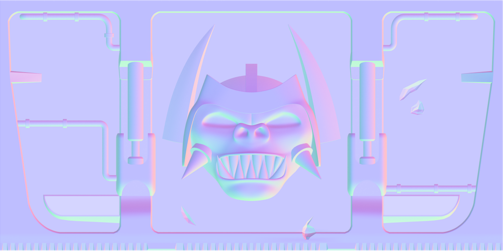
I’m using these images taken from the excellent Duke3D High Resolution Pack (HRP) for educational purposes. Although we could’ve generated the bump map using the technique from my previous post, this especially-tailored bump map will provide better results.

Believe it or not, there are no more input textures used! The final image was produced by applying the technique on these two. This is the reason I think bump mapping is such a game changer. This technique alone can significantly up the quality and realism of the images our renderers produce.

It is especially shocking when we compare the diffuse map with the final bump-mapped image. Even if we applied per-pixel lighting to the diffuse map in our rendering pipeline, the results would be nowhere close to what we can achieve with bump mapping. Bump mapping really makes this door “pop out” of its surface.

Bump Mapping Theory

The theory I develop in these sections is heavily based on the books Mathematics for 3D Game Programming and Computer Graphics from Eric Lengyel and More OpenGL from David Astle. You should check those books for the definitive reference on bump mapping. Here, I try to explain the concepts in simple terms.

So far, you might have noticed I’ve been mentioning that the bump map consists of the “deformed” normals that we should use when applying the lighting equation to the scene. But I haven’t mentioned how these normals are actually introduced into our lighting equations.

Remember from my previous post how we mentioned that normals are stored in the RGB image? Remember that normals close to (0,0,1) looked blueish? Well, that is because normals are stored in a coordinate system that corresponds to the image. This means that, unfortunately, we can’t just take each normal N and plug it into our lighting equation. If we call L the vector that takes each 3D point (corresponding to each fragment) to the light source, the problem here is that L and N are in different coordinate systems.

L is, of course, in camera or world space, depending on where you like doing your lighting math. But where is N? N is defined in terms of the image. That’s neither of those spaces.

Where is it then? Well, N is actually in its own coordinate system that authors refer to as “tangent space”. It’s its own coordinate system.

In order to apply per-pixel lighting using the normals coming from the bump map, we’ll have to bring all vectors to the same coordinate system. For bump mapping, we usually bring the L vector into tangent space instead of bringing all the normals back into camera/world space. It seems more convenient and should produce the same results.

Once L has been transformed, we will retrieve N from the bump map and use the Lambert equation between these two to calculate the light intensity at the fragment.

From World Space to Tangent Space

How can we convert from camera space to tangent space? Tangent space is not by itself defined in terms of anything that we can map to our mesh. So, we will have to use one additional piece of information to determine the relationship between these two spaces.

Given that our meshes are composed of triangles, we will assume the bump map is to be mapped on top of each triangle. The orientation will be given by the direction of the texture coordinates of the vertices that comprise the triangle.

This means that if we have a triangle that has an edge: (-1,1)(1,1) with texture coordinates: (0,1)(1,1), a horizontal vector (1,0) represents a vector tangent to the vertices that is aligned with the horizontal texture coordinates. We will call this the tangent.

Now, we need two more vectors in order to define the coordinate system. Well, the other vector we can use is the normal of the triangle. This vector is, by definition, perpendicular to the surface and will be perpendicular to the tangent.

The final vector we will use to define the coordinate system has to be perpendicular to both, the normal and the tangent, so we can calculate it using a cross product. There is an ongoing debate whether this vector should be called the “bitangent” or the “binormal” vector. According to Eric Lengyel the term “binormal” makes no sense from a mathematical standpoint, so we will refer to it as the “bitangent”.

Now that we have three vectors that define the tangent space, we can create a transformation matrix that takes vector L and puts it in the same coordinate system that the normals for that specific triangle. Doing this for every triangle will allow applying bump mapping on the triangle.

Responsibility – who does what

Although we can compute the bitangent and the transform matrix in our vertex shader, we will have to supply the tangent vectors as input to our shader program. Tangent vectors need to be calculated using the CPU, but (thankfully) only once. Once we have them, we supply them as an additional vertex array.

Calculating the tangent vectors is trivial for a simple surface like our door, but can become very tricky for an arbitrary mesh. The book Mathematics for 3D Game Programming and Computer Graphics provides a very convenient algorithm to do so, and is widely cited in other books and the web.

For our door, composed of the vertices:

(-1.0, -1.0, 0.0)
(1.0, -1.0, 0.0)
(1.0, 1.0, 0.0)
(-1.0, 1.0, 0.0)

Tangents will be:

(1.0, 0.0, 0.0)
(1.0, 0.0, 0.0)
(1.0, 0.0, 0.0)
(1.0, 0.0, 0.0)

Once we have the bitangents and the transformation matrix, we rotate L in the vertex shader, and pass it down to the fragment shader as a varying attribute, interpolating it over the surface of the triangle.

Our fragment shader can just take L, retrieve (and decode) N from the bump map texture and apply the Lambert equation on both of them. The rest of the fragment shading algorithm need not be changed if we are not applying specular highlights.

In Conclusion

Bump mapping is an awesome technique that greatly improves the lighting in our renderers at limited additional costs. Its implementation is not without a challenge, however.

Here are the steps necessary for applying the technique:

• After loading the geometry, compute the per-vertex tangent vectors in the CPU.
• Pass down the per-vertex tangents as an additional vertex array to the shader, along with the normal and other attributes.
• In the vertex shader, compute the bitangent vector.
• Compute the transformation matrix.
• Compute vector L and transform it into tangent space using this matrix.
• Interpolate L over the triangle as part of the rasterization process.
• In the fragment shader, normalize L.
• Retrieve the normal from the bump map by sampling the texture. Decode the RGBA values into a vector.
• Apply the Lambert equation using N and the normalized L.
• Finish shading the triangle as usual.

On the bright side, since this technique doesn’t require any additional shading stages, it can be implemented in both OpenGL and OpenGL ES 2.0 and run on most of today’s mobile devices.

In my next post I will show bump mapping applied to a 3D model. Stay tuned!